Research
Current Interests
- Putting machine learning in production
- Search Relevance
- Large scale data processing
- Successful data science projects
- Data product teams and organizations
- Building data teams
- Data strategy and creating data driven products
Past Research Interests
- social media analysis, data science
- reinforcement learning, adaptive control
- machine learning, statistical learning theory
- kernel methods
- feature extraction
- machine learning for multimedia data
- clustering, stability based model selection
- approximation theory for eigenvalues and eigenvectors
- programming languages for machine learning
- some bioinformatics, brain-computer interface
"Political" Interests
- open source software for machine learning
- interoperatibility of ML software
- reproducibility of ML research
Activities
Sören Sonnenburg, Cheng Soon Ong, and I have initiated a novel track for machine learning software within the Journal of Machine Learning Research, for which we now function as action editors. We have also set up a website as a repository for resources on machine learning open source software.
I have co-organized (together with Sören Sonnenburg, Cheng Soon Ong, and S.V.N. Vishwanathan a workshop on open source software for machine learning at this years NIPS conference (MLOSS).
Stefan Harmeling and I are playing around with designing a new programming language, called rhabarber. The language should be specifically tailored to machine learning. Currently it's in what one would call "pre-alpha", and several major design changes are planned for this summer, but if you're curious, you can find more information on the project homepage.
Projects
Here is a short list of the projects I've already worked on. ("Worked on" means that I was paid by these projects, and/or was responsible for the part of the project of the respective institution.)
University of Bonn (1995-2004)
- Retina Implant project Building an adaptive neuronal implant for people suffering from retinitis pigmentosa, a disease which ultimately leads to blindness.
- emilea e-stat A project aimed at building an environment for e-learning. The university of Bonn was a content-provider for machine learning.
- Teaching duties.
Fraunhofer Institute FIRST (2004-2007)
- A project together with Daimler-Chrysler to measure the amount of mental workload of a car driver using EEG.
- ADDnet Finding new methods for detecting proteinurea in an early stage using bioinformatics. This was an EU project headed by the University of Helsinki
- FaSor An extension of the earlier project with Daimler-Chrysler. The goal is to interpret the driver as a sensory system.
- THESEUS A large project funded by the Bundeswirtschaftsministerium. I was responsible for designing the part of Fraunhofer FIRST. Our task will be to automatically extract semantic annotation for images.
Technical Universtiy of Berlin (2007-2019)
Technically, my position is paid for by the university (Haushaltsstelle), so I'm not on the payroll of any specific project.
- Teaching duties.
- A bit of system administration.
- ALICE - Autonomous learning in complex environments. Joint project with Siemens and idalab GmbH with applications to wind turbine control.
TWIMPACT/streamdrill (2010-2014)
TWIMPACT, later streamdrill, was my start-up-on-the-side. It was concerned with real-time social media stream analysis.
Fedistats (2023-)
Fedistats is a news aggregation and trend analysis project based on Mastodon.
Research Topics

Twimpact
Micro-blogging services like twitter have become very popular in recent years. As of now, exploring such services and finding interesting users is still an open problem.
With our project twimpact we explore methods for automatically measuring user impact, or studying the network structure of micro-blogging services.
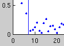
On Relevant Dimensions in Kernel Feature Spaces
It is well known that using a kernels for supervised learning corresponds to mapping the problem into a potentially quite high-dimensional feature space. Usually, complexity control (for example, large margin hyperplanes) is attributed with the fact that learning is still possible. We showed, however, that using the right kernel leads to a typically small effective dimensionality in a feature space, meaning that even in infinite-dimensional feature spaces, the learning problem is in fact contained in a low-dimensional subspace.